Using Matrices to Solve Linear Systems

A linear system can be solved using matrices. Each row in the matrix represents one linear equation. Each column in the matrix represents a variable in the linear equations.

Transforming a Linear System to a Matrix

Start with the linear system

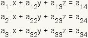
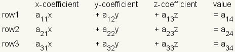
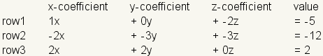
where is a coefficient. Organize the linear system by variable for columns and equations for rows:

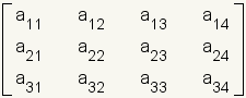
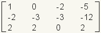
Now drop the variables and operators and draw matrix brackets around the values:

Example: Start with the linear system

Now organize it into rows and columns. Now put the system into matrix notation.

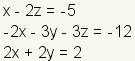Row Operations

There are row operations that can be done on a matrix that, if done correctly, will help transform the matrix into a solution to the linear system represented by the matrix. These operations are:

• Scalar multiplication of a row: Any row can be multiplied by any nonzero real number.
• Row addition: Any row can be added to any other row and the sum be used to replace either row.
• Trading rows: Any two rows can be swapped.

Scalar Multiplication of a Row

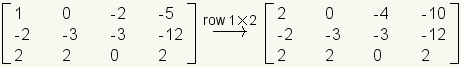
Scalar multiplication of a row is like scalar multiplication of the entire matrix, but it is done to only one row. In the following example, row 1 is multiplied by 2.

When multiplying rows, it is usually best to use whole numbers whenever possible. This makes later steps in solving the linear system much easier.

Addition of Rows

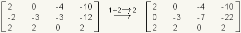
When adding rows, corresponding elements of each row are added together. The results are placed into either of the rows being added. In the following example, row 1 is added to row 2 and the result placed into row 2.

Note that the first entry in row 2 is now zero. As you will see as you follow this algorithm, this was the goal of the first operations on this matrix.

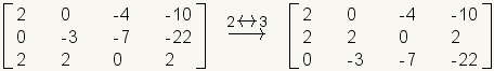
Swapping Rows

Any two rows in the matrix can be swapped without changing the linear system represented by the matrix. While row swapping is not necessary for solving this sample system, it is demonstrated here by swapping rows 2 and 3.

Row swapping to solve linear system is usually used to move a row with leading zeros into a more convenient spot in the matrix.

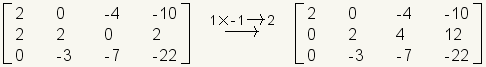
Combining Operations

Any of the operations can be combined into a single transformation of the matrix. Be careful though, the more complicated combinations of transformations can lead to errors. Any error will give false results. In the next example, row 1 is multiplied by negative 1 and added to row 2.

The Algorithm

Each of the steps in this algorithm are completed using the row operations of scalar multiplication of rows, addition of rows, and swapping rows.

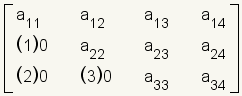
The first step in solving a linear equation using a matrix is to get all zeros below the diagonal. The order in which these are conventionally done is illustrated here:

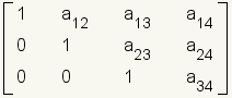
The second step is to transform the matrix so that the coefficients in the diagonal are all ones. This is illustrated by the following matrix.

This is called row-echelon form. A matrix representing a linear system that is in row-eschelon form can be solved the rest of the way by using back substitution. Solving a matrix this way is called Gaussian elimination.

The third step is to transform the matrix so entries above the diagonal are all zeros. The following matrix illustrates this step.

Once the matrix is in this form, called reduced row-echelon form, the solution can be read off the matrix: Solving a matrix this way is called Gauss-Jordan elimination.

Example (continued)

Divide both row 1 and row 2 by 2. This makes them easier to work with.

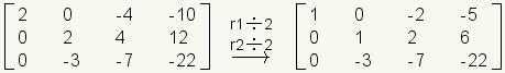Multiply row 2 by 3 and add it to row 3.

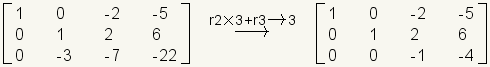Multiply row 3 by -1.

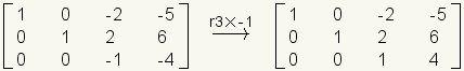Multiply row 3 by -2 and add it to row 2 with the result in row 2.

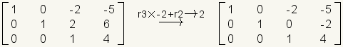Multiply row 3 by 2 and add it to row 1 with the result in row 1.

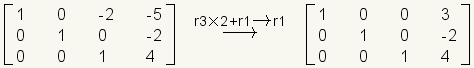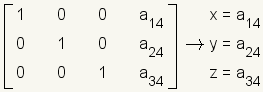
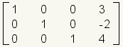
Read the solution from the matrix.

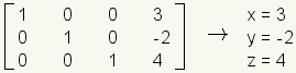Classes of Solutions

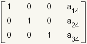
Exactly one solution: A linear system with exactly one solution will have a diagonal of ones, and the rest zeros except for the rightmost column:

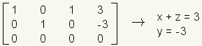
Infinite solutions: A linear system with infinite solutions will have a row of all zeros, and can not be reduced to reduced eschelon form:

No solution: A linear system with no solution will have a row with all zeros except for the last entry. This is the mathematical statement 0=7, which is impossible. So there is no solution.

Cite this article as:

McAdams, David E. Using Matrices to Solve Linear Systems. 12/17/2018. All Math Words Encyclopedia. Life is a Story Problem LLC. https://www.allmathwords.org/en/m/matrixlinearsystem.html.

Image Credits

• All images and manipulatives are by David McAdams unless otherwise stated. All images by David McAdams are Copyright © Life is a Story Problem LLC and are licensed under a Creative Commons Attribution-ShareAlike 4.0 International License.

Revision History

12/17/2018: Removed broken links, updated license, implemented new markup. (McAdams, David E.)
8/28/2018: Corrected spelling. (McAdams, David E.)
8/7/2018: Changed vocabulary links to WORDLINK format. (McAdams, David E.)
12/23/2008: Corrected spelling. (McAdams, David E.)
12/16/2008: Initial version. (McAdams, David E.)