Probability

Pronunciation: /ˌprɒb.əˈbɪl.ɪ.ti/ Explain

Probability is the likelihood of an event happening. Some other synonyms for probability are chance and odds. When you say, "I'll probably be at school tomorrow," you are saying it is likely you will be at school tomorrow, that there is a good chance you will be at school tomorrow.

Notation

The notation P( A ) is used to show probability. To write that the probability of rain is 50%, write P(rain) = 0.5. Notice that a decimal number is used, not a percentage.

In probability, we talk about or use:

• Event: An occurrence about which probability is measured, calculated, or estimated.
• Experiment: An experiment is doing something that makes an event occur.
• Outcome: An outcome is one way an event can occur.
• Sample space: A sample space is all of the possible outcomes.
• Probability function: A function that, when given an event, returns an estimated or actual probability of that event occurring. If one adds together the probability of all events, the sum must be 1 since this reflects all possibilities.
• Probability distribution graph: A graph that shows how the probability of events is distributed over the sample space.

Example 1: Flipping a Coin

When one flips a coin and records the result, one is doing an experiment in probability. The parts of the experiment are: Part Description Experiment The experiment is the whole process of flipping the coin and recording the event. Event The event is flipping the coin. Outcome The outcome is either heads or tails. Sample Space The sample space is heads and tails. One can write this in set notation as {heads, tails}. 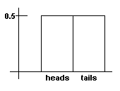Probability Function P(heads) = 0.5, P(tails) = 0.5. This means that half the time (0.5 = 1/2), the coin comes up heads and half the time it comes up tails. The sum of all the possibilities is 0.5 + 0.5 = 1 P( x ) Possible Combinations Fraction Decimal P( H ) 1/2 0.5 P( T ) 1/2 0.5 Probability Distribution Graph Figure 1: Probability distribution of a coin flip. This probability distribution graph represents how the probability of each event is distributed over the whole sample space. In this case the odds of heads is just the same as the odds of tails.

Example 2: Flipping Two Coins

When one flips both coins and records the result, one is doing an experiment in probability. The parts of the experiment are: Part Description Experiment The experiment is the whole process of flipping both coins and recording the event. Note that this could also be done by flipping the same coin twice. Event The event is flipping both coins. Outcome The outcome is one of: both heads, heads thentails, tails then heads, or both tails. This can be abbreviated as HH, HT, TH, and TT where 'H' stands for heads and 'T' stands for tails. Sample Space There are 4 outcomes in the sample space. In set notation this is {HH, HT, TH, TT}. 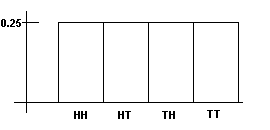Probability Function P(HH)=0.25, P(HT)=0.25, P(TH)=0.25, P(TT)=0.25. Each of the four outcomes have the same likelihood, or probability, of occurring. So the probability of each is 1/4 = 0.25. The sum of all the possibilities is 0.25 + 0.25 + 0.25 + 0.25 = 1.0. P(x) Possible Combinations Fraction Decimal P(HH) 1/4 0.25 P(HT) 1/4 0.25 P(TH) 1/4 0.25 P(TT) 1/4 0.25 Probability Distribution Graph Figure 2: Probability distribution of flipping two coins This probability distribution graph represents how the probability of each event is distributed over the whole sample space. In this case the odds each of the outcomes is equal. What if one does not care which coin comes up heads and which coin comes up tails? Then a tails then a heads (TH) is the same as a heads then a tails (HT). This means that there are 3 outcomes: HH, HT, TT. The parts of the experiment then are: Part Description Experiment The experiment is the whole process of flipping both coins and recording the event. Note that this could also be done by flipping the same coin twice. Event The event is flipping both coins. Outcome The outcome is one of: both heads, heads and tails, or both tails. This can be abbreviated as HH, HT, and TT where 'H' stands for heads and 'T' stands for tails. Sample Space There are 3 outcomes in the sample space. In set notation this is {HH, HT, TT}. 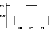Probability Function P(HH)=0.25, P(HT)=0.5, P(TT)=0.25. Since there is a one in four chance ( P = 0.25) of a heads then a tails and a one in four chance of a tails then a heads, when these are combined together, we add 0.25 + 0.25 = 0.5. The sum of all the possibilities is 0.25 + 0.5 + 0.25 = 1. P(x) Possible Combinations Fraction Decimal P(HH) 1/4 0.25 P(HT) or 1/2 0.5 P(TT) 1/4 0.25 Probability Distribution Graph Figure 3: Probability distribution of flipping 2 coins. This probability distribution graph represents how the probability of each event is distributed over the whole sample space. In this case the odds each of the outcomes is not equal.

Example 3: Rolling two dice

Now take a look at rolling two dice. Usually one does not care which die has which value. One only cares about the sum of the dice. Part Description Experiment The experiment is the whole process of rolling the two dice and recording the event. Note that this could also be done by flipping the same coin twice. Event The event is rolling two dice. Outcome Since one cares only about the total of the two dice, the outcome is one of the following: 2, 3, 4, 5, 6, 7, 8, 9, 10, 11, 12. Sample Space There are 11 outcomes in the sample space, 2 through 12. In set notation this is {2, 3, 4, 5, 6, 7, 8, 9, 10, 11, 12}. 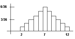Probability Function The probability function for this experiment is: P(x) Possible Combinations Fraction Approx Decimal P(2) 1/36 0.0278 P(3) , 2/36 0.0556 P(4) , , 3/36 0.0833 P(5) , , , 4/36 0.1111 P(6) , , , , 5/36 0.1389 P(7) , , , , , 6/36 0.1667 P(8) , , , , 5/36 0.1389 P(9) , , , 4/36 0.1111 P(10) , , 3/36 0.0833 P(11) , 2/36 0.0556 P(12) 1/36 0.0278 Adding all the probabilities together gives: 36/36 = 1. Probability Distribution Graph Figure 4: Probability distribution for rolling 2 six-sided dice. This probability distribution graph represents how the probability of each event is distributed over the whole sample space. In this case the odds each of the outcomes is not equal.

Principles of Probability

Four basic principles of probability are:

1. When quantifying, or saying the value, of a probability, we use a number between 0 and 1. In algebraic notation, for an arbitrary event A, 0 ≤ P(A) ≤ 1.
2. The probability of an impossible event is 0. If event E is impossible, we write P( E ) = 0. This means that the probability of E occurring is exactly 0. In real life, very few events are absolutely impossible.
3. The probability of an event that will certainly happen is 1. If event H is certain, we write P(H) = 1.
4. The probability of an event not happening is 1 less the probability of that event happening. In algebraic notation for an arbitrary event A: P(!A) = 1 - P(A). For example, if there is a 30% chance of rain today we write P(rain) = 0.3. This means that the chance of rain not occurring today is P(no rain) = 1 - P(rain) = 1 - 0.3 = 0.7.

References

1. McAdams, David E.. All Math Words Dictionary, probability. 2nd Classroom edition 20150108-4799968. pg 144. Life is a Story Problem LLC. January 8, 2015. Buy the book
2. Grinstead, Charles M. and Snell, J. Laurie. Introduction to Probability. http://www.dartmouth.edu/~chance/teaching_aids/books_articles/probability_book/amsbook.mac.pdf. Buy the book
3. Ross, Sheldon. A First Course in Probability. 6th edition. Pearson Education. 2002. Buy the book

More Information

• McAdams, David E.. Probability. lifeisastoryproblem.com. Life is a Story Problem LLC. 3/12/2009. http://www.lifeisastoryproblem.com/probability/index.html.

Cite this article as:

McAdams, David E. Probability. 4/28/2019. All Math Words Encyclopedia. Life is a Story Problem LLC. https://www.allmathwords.org/en/p/probability.html.

Image Credits

• All images and manipulatives are by David McAdams unless otherwise stated. All images by David McAdams are Copyright © Life is a Story Problem LLC and are licensed under a Creative Commons Attribution-ShareAlike 4.0 International License.

Revision History

4/28/2019: Changed equations and expressions to new format. (McAdams, David E.)
12/21/2018: Reviewed and corrected IPA pronunication. (McAdams, David E.)
12/1/2018: Removed broken links, updated license, implemented new markup. (McAdams, David E.)
8/7/2018: Changed vocabulary links to WORDLINK format. (McAdams, David E.)
1/12/2010: Added "References". (McAdams, David E.)
6/7/2008: Corrected spelling. (McAdams, David E.)
4/14/2008: Added probability distribution graphs. (McAdams, David E.)
4/12/2008: Simplified wording. Reorganized article. Expanded article with examples (McAdams, David E.)
3/22/2008: Revised See Also to match current specification. (McAdams, David E.)
7/12/2007: Initial version. (McAdams, David E.)